Tutorials

On this page, several tutorials are listed explaining the usage of VOLPES through several hands-on examples that can be followed along using the app itself. The tutorial examples are ordered roughly according to increasing difficulty and complexity, but can be read in any order.

Comparing two hydrophobicity scales

Step 1

When starting an analysis, the user is greeted with a nearly empty page showing a single button, asking the user to run an analysis. Clicking this button opens up the Settings menu to start defining a sequence and the parameters for analysis.

Step 2

The opened Options dialogue shows several tabs that guide the user through data submission process in a meaningful order. First sequence data is defined. This is followed by the definition of the scale used and finally the visual style is set.

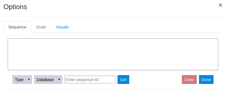
Step 3

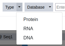
Sequence information can be provided in multiple ways: the sequence can be entered directly in the textbox (as a raw string of one letter encoded amino acids or bases, or FASTA formatted), or it can be retrieved by using the ID of a public sequence database. For this example, the latter option is chosen. First, the type of polymer is defined - in this case a protein sequence.

Step 4

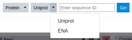
Selecting a molecule type automatically selects the corresponding database, that is available for sequence download. Two large public sequence databases are supported currently: the Uniprot¹ for proteins and the European Nucleotide Archive (ENA)² for RNA/DNA sequences. This tutorial example, uses a protein sequence deposited in the Uniprot database.

Step 5

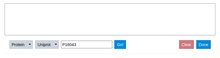
To access a deposited sequence, the ID is simply inserted into the input field provided and the Go button to the right is clicked.

Step 6

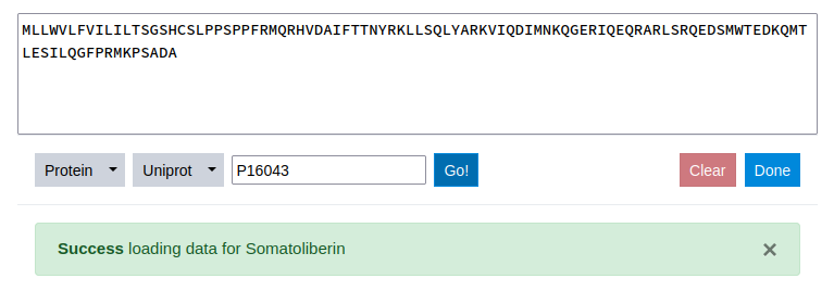
Once a sequence ID is submitted, the data is automatically retrieved from the specified server. The sequence itself is inserted in the text-editor that allows for further modification of the sequence and a success message is displayed mentioning the name of the protein sequence. The Clear button to the left of the Done button allows for deletion of all specified data.

Step 7

Once the sequence is loaded, the first step is done. Next a property of interest needs to be selected. To do this the Scale tab is clicked.

Step 8

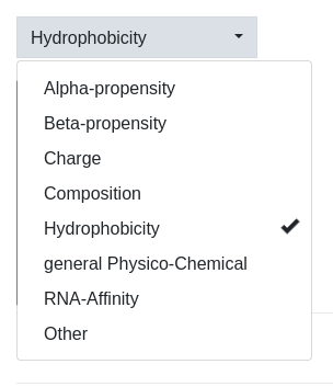
Within the Scale tab a dropdown-menu is found that allows to prefilter the scales in a coarse way. This is necessary since over 600 different property scales are supplied with the tool. In our case, we want to compare the hydrophobic pattern as defined by two different scales and, therefore, only the Hydrophobicity option is selected. This filter allows for multiple classes to be selected.

Step 9

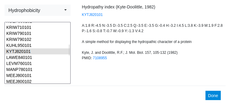
Once one or more classes are selected, the menu gets populated with all scales fitting the selected class(es). They are listed using their AAindex ID³ if available or a descriptive name otherwise. First, a very popular scale, the Kyte-Doolittle Hydropathy index, is selected. Immediately, the data on the right gets updated showing the name, a link to the AAindex (if applicable), the numerical entries of the scale, a short description and a citation for the original publication, including a link to the Pubmed if available.⁴

Step 10

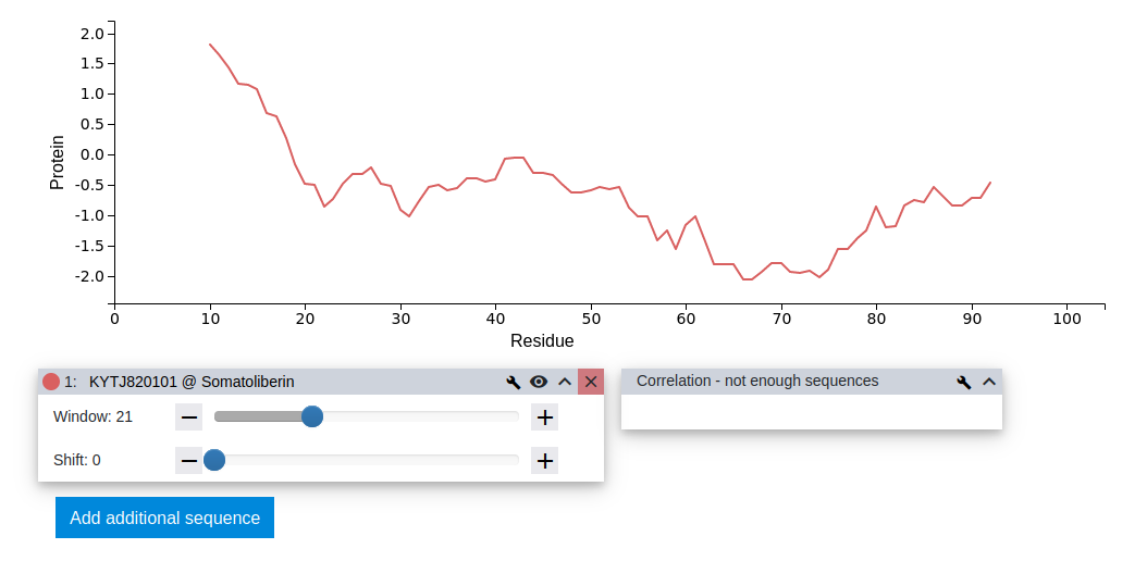
For now, the visual parameters are kept at their default values and the resulting profile is investigated. To do that, the pop-up is closed by clicking the Done button on the bottom right. A distinct hydrophobic profile can be observed showing positive values at the N-terminus of the sequence and the most negative region closer towards the C-terminus of the protein.

Step 11

To be able to compare two different scales, the same sequence is added a second time using the Add additional sequence button. Steps 2 to 8 are repeated again using the Uniprot ID P16043 to download the sequence of Somatoliberin from the Uniprot database.

Step 12

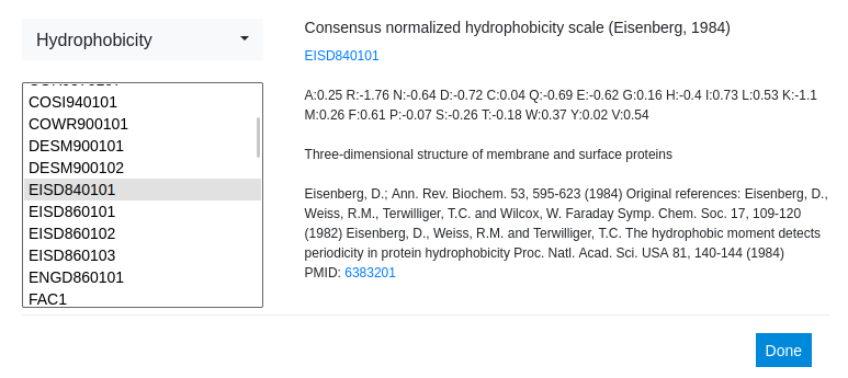
This time another well-known hydrophobicity scale is used: the Consensus normalized hydrophobicity scale by Eisenberg et. al. Already at this step a difference in absolute values between the two scales can be observed in the description of the scale.

Step 13

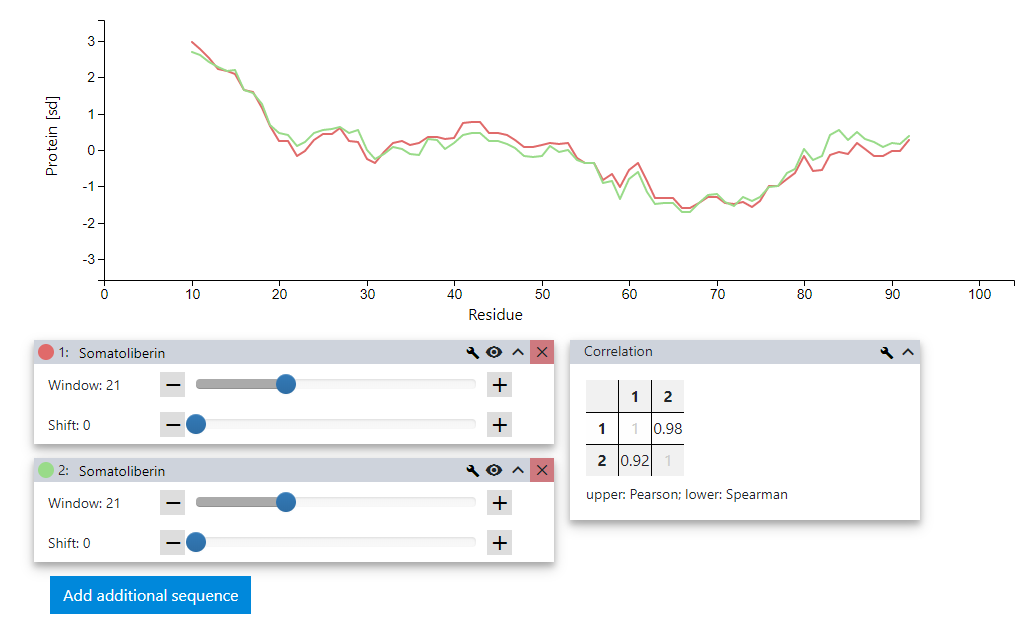
Once the second dataset is defined, the resulting plot can be investigated. While the profiles suggest little similarity, the pairwise Pearson correlation coefficient R between them is 0.98, suggesting a very high correlation. This can happen if two scales are reporting their properties in correlated, but largely different units.

Step 14

To test whether the difference between the two curves can be purely attributed to differences in units used by the scale authors, we can normalize the profiles by their standard deviation. To do so, we click the Settings button in the top menu bar.

Step 15

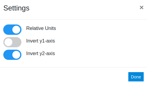
In the settings menu the Relative Units switch is flipped to on, this recalculates the profiles and reports them in units of their own standard deviation. The other options allows one to invert the y-axes, which can be useful if one compares properties that are reported in inverted units.

Step 16

Once the settings menu is closed, the similarities between the two profiles for Somatoliberin using two different hydrophobicity metrics are obvious. The differences between the two scales used seem to be very local in nature with the global shape staying intact.

This example illustrates a simple task performed using VOLPES, of course VOLPES can do much more than what is described above, but this should be enough to get you started!

Aligning alternative splicing variants

Step 1

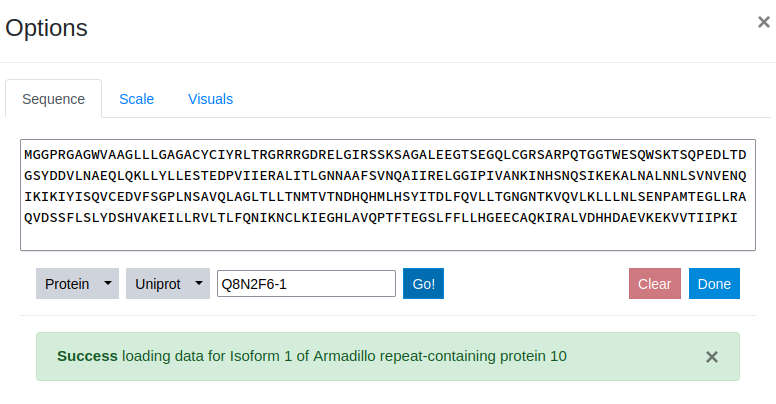
We start by adding the first protein sequence Armadillo repeat-containing protein 10 using the Uniprot ID Q8N2F6-1. Note that the "-1" indicates a splicing isoform, in this case we selected the canonical sequence.

Step 2

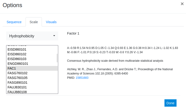
For this example we want to compare the variants based on hydrophobicity - therefore we choose the FAC1 scale. Factor 1 is a consensus hydrophobicity scale derived by multivariate statistical analysis of a set of 500 different property scales.

Step 3

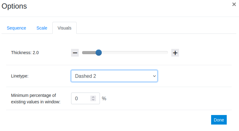
Next we add a splicing variant using the Uniprot ID Q8N2F6-2. To do this we repeat steps 1-2 using the second ID. This time we want to make sure the alternative sequence stands out in the plot. To achieve that we switch to the Visuals tab and change the linetype to a style of our choice, in this example: Dashed 2. In addition to the linetype and thickness, in this tab the minimum percentage of values that have to be present in an averaging window can be adjusted. For details on this parameter, see Documentation.

Step 4

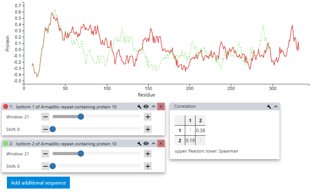
The similarity between the two sequences is not immediately obvious, neither by the plot nor by the Pearson or Spearman correlation coefficients displayed in the lower right tab.

Step 5

To make sure that we are not missing anything we start sliding the profiles against each other by using the Shift slider of the second sequence. To fine tune the shift the + and - buttons next to slider can also be used. When reaching an offset of 35 residues the similarity between the two variants becomes very obvious. A look at the correlation tab confirms that these sequences are highly similar.

Using the tools provided by VOLPES we could quickly and easily find the overlapping regions for these two splicing isoforms.